Quick pre-stack seismic inversion to predict reservoir properties at a gas and condensate field in Nam Con Son basin
Summary
This paper introduces a new approach to quickly predict reservoir quality along a particular directional well-path, to justify the optimisation process for well location. The workflow employs a simulated annealing algorithm to convert available seismic data at well locations into some petrophysical properties that indicate reservoir quality such as porosity and water saturation. The inversion process is constrained by several seismic traces that are previously extracted along the well-path, which help significantly reduce the calculation cost. The results were successfully applied in two development wells drilled into gas bearing reservoirs in Nam Con Son basin, offshore Vietnam.
Key words: Reservoir quality, seismic inversion, rock physics model, Vshale, porosity, water saturation, Nam Con Son basin.
1. Introduction
Seismic inversion (post- and pre-stack) is widely used in reservoir characterisation [1 - 4]. The basic idea is to relate changes in rock properties due to hydrocarbon introduction into the formation to the changes in pre-stack seismic amplitude via a mathematical equation, which is also called a rock physics model. The model is then used to convert rock properties (porosity, saturation, shale content) into some common seismic properties (velocity, density, Poisson ratio) [4], which are further used to predict other properties via cross-plot or some mathematical approaches such as neural network or multi-attribute cross-plots [5 - 7].
A gas and condensate field in Nam Con Son basin is recently developed to produce hydrocarbon from Miocene reservoirs. Geophysical studies show strong AVO responses at reservoir levels, which indicate hydrocarbon saturated sands.
The fluid replacement modelling using Gassmann fluid substitution equation showed significant reduction of offset amplitude when gas replaces water within the reservoir bodies (Figure 1).
 |
Figure 1. Fluid replacement modelling shows improved AVO anomalies of gas replacing water
Intense in-house qualitative studies [8] have been carried out to understand the reservoirs, including AVO classes, fluid factors indicator, and the AB fluid factor (ABFF) to help improve the interpretation and well target optimisation. In Figure 2, the ABFF attribute successfully highlights the fluid existence in reservoirs A1 and F1.
 |
Figure 2. ABFF attribute highlights fluid potential of reservoirs A1 and F1
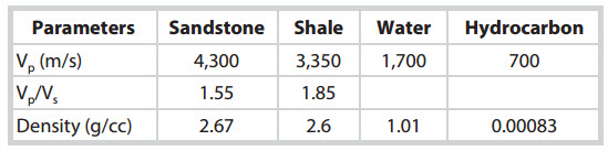 |
Table 1. Input petrophysical parameters for the rock physics model
 |
Figure 3. Excellent correlations in QC plot of the input rock physics model
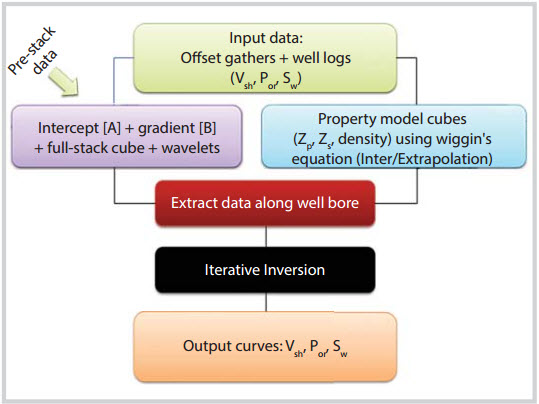 |
Figure 4. Inversion flow chart
Seismic inversion is practically employed to quantitatively predict reservoir properties at candidate well locations. The common approach is performed on the trace by trace basis, which is suitable for nearly vertical well-path as a single run could provide sufficient information to the whole well-path. However, since most wells in the field are deviated, it requires many seismic traces to cover the well profiles, consequently increasing the calculation cost. A new approach is proposed to quickly estimate the interested properties and help save the decision making time.
2. Method
The approach employs Wyllie’s linear approximation equation [9] as a rock physics model to connect the petro-physical properties - porosity
(PHI), water saturation (Sw) and the shale content (Vsh) - to geophysical parameters such as velocity (P-wave Vp and S-wave Vs) and density. The latter set of parameters is then used to convert into synthetic responses using the re-written three-term Aki- Richard approximation by Wiggins et al. [10]. Below is a set of Wyllie approximation equation used in our method:

Where:
Vpst, VpSh, Vpw, VpHC are P-wave velocities of pure sandstone framework, pure shale, water and hydrocarbon;
Dn , Dn , Dn , Dn are densities of pure sandstone framework, pure shale, water and hydrocarbon.
The parameters used at this field are listed as in Table 1. Figure 3 shows the comparison between the estimated Vp, Vs and density curves (red line) with the actual recorded log (green line). Excellent matches between corresponding curves validate the above rock physics model.
The simulated annealing algorithm [3, 11] is used to invert the pre-stack seismic data. This global optimisation process takes into account a low frequency model and perturbs it to find the best fit model that satisfies the seismic responses. The outputs are a best fit model and many other fit models that can be used for uncertainty analyses. In this study, we use the best fit model for final prediction values. Figure 4 summarises the general workflow of the inversion algorithm.
The low frequency starting models are generated by interpolating logs from available wells nearby, and applying a low frequency filter to retain the low frequency content. Figure 4 demonstrates the inversion flow chart template.
The inversion is expected to output three parameters. In order to remove the non-uniqueness in the solution, the input seismic data has to be of multiple traces. Therefore, pre-stack data is required.
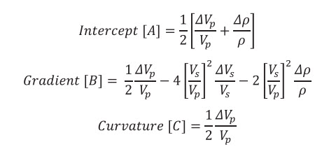
The common pre-stack inversion involves comparing synthetic to real angle gather traces to update the input to satisfy the real data [4, 12]. However, this is very time- consuming considering many angle traces involved in the calculation process at each location. For this approach, to reduce the computing cost, we convert the NMO corrected offset volume into intercept, gradient and curvature volumes using an input stacking velocity cube [4]. The intercept corresponds to seismic response of a zero offset trace, the gradient and curvature reflect how amplitude changes with offset.
Due to the limitation of data acquisition parameter, the pre-stack volume is limited to 30 degree angle offset for usable quality. With this limited angle range, the effect of the curvature term on the overall inversion results is minimal. Meanwhile, the final stack volume, which is a summation product of the intercept, gradient and curvature, is still showing a strong effect on the inversion results. Therefore, we use the full-stack volume along with the intercept and gradient volumes for inversion constraint. To perform the inversion at deviated wells, we first extract those parameters along the well-paths and input them into the algorithm.
Three synthetic traces created by using the equation of Wiggins et al. [10] are compared against the corresponding traces from real data to control the inversion algorithm. Below Wiggins’ equations are used to generate synthetic traces for error calculation.

Where:
3. Results
We successfully applied the method to a drilled nearly vertical exploration well (well-X) for quality control and on two other development locations (wells P1 and P2) with very close results from final LWD petrophysical analyses.
The nearly vertical exploration well (well-X) indicated gas bearing for two target reservoirs: a gas saturated sand A1 of 15mTVD thickness with 26% porosity, 20% average water saturation and 5% shale volume (Vsh); a massive gas and condensate saturated sand F1 of 36mTVD thickness with 14% porosity, and 46.9% average water saturation. In Figure 5, the inverted results (dark blue) have excellent matches in stack, intercept and gradient traces, while the porosity, Sw and Vshale, fit very well with actual curves calculated from well logs (red). The estimated Vshale and porosity curves even give accurate prediction of the layering from the changes in values. This encourages us to apply the approach to predict at other deviation well locations.
At the first development location, well-P1 targeting both A1 and F1, maximum 33o deviated profile, the synthetic traces match excellently with the input traces (Figure 6). The inversion predicted very well the properties, with almost perfect match of the logs of A1; excellent matches of porosity and Vshale and average match of the water saturation of the F1. With the latter reservoir, the algorithm also predicted layering via fluctuations of porosity and Vshale curves. The actual drilling results confirm this point.
On the second development well-P2, targeting reservoir F1 with maximum 42o deviated profile, the inversion predicted reservoir existence at target locations, with high correlations with actual seismic traces. However, the estimated properties are poorer than the actual well results of the F1 interval (Figure 7). This suggested the heterogeneity of F1 properties from well-X location, such as changes in signatures of Vshale and Sw (much lower readings). Since the prediction is dependent of the input model, which is controlled by the well-X properties, the error is reasonable.
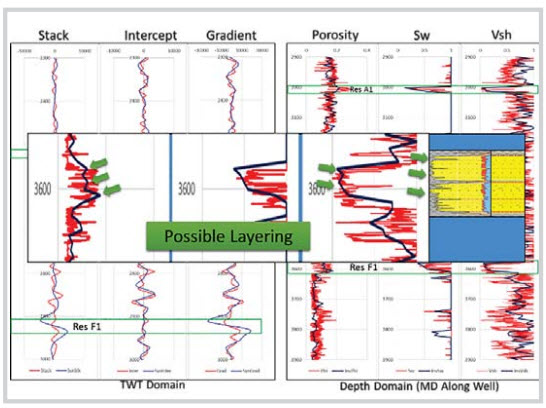 |
Figure 5. Inverted dark blue curves having excellent matches with input seismic traces and actual logs (red curves) at well- X
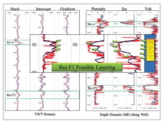 |
Figure 6. Inverted dark blue curves with excellent matches with input seismic traces and actual logs (red curves) at well- P1
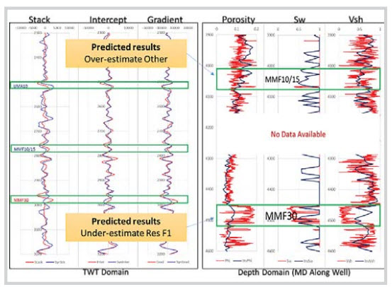 |
Figure 7. Inverted dark blue curves with having excellent matches with input seismic traces but average matches with actual logs (red curves) at well- P2
4. Conclusion
The introduced method offers a quick-look prediction of reservoir quality along a proposed deviated well path by directly inverting the seismic data into reservoir properties. It requires a starting model acting as an initial guess, guiding the algorithm to the optimal result that satisfies seismic traces extracted along the well-bore. The starting model can be generated from interpreted petrophysical parameters of a nearby well.
This method is proven to be reliable at well locations within homogeneous area. However, for highly heterogeneous reservoirs, the method will not well predict the properties unless proper guidance of the geological heterogeneity is given to the input model.
At the current stage, the algorithm is working along a particular well-path. In case there are enough controlling wells, the algorithm could be used for 3D volumes for spatial mapping of reservoir properties.
Acknowledgement
We thank the Vietnam Oil and Gas Group and Bien Dong POC for allowing us to use the data and publish the results.
Reference
1. Albert Tarantola. Inversion of seismic eflection data in the acoustic approximation. Geophysics. 1984; 49(8): p. 1259 - 1266.
2. Brian Russell, Dan Hampson. A comparison of post-stack seismic inversion methods. SEG Technical Program Expanded Abstracts. 1991: p. 876 - 878.
3. Mrinal K.Sen, Paul L.Stoffa. Global optimization methods in geophysical inversion. Elsevier Science Publications, Netherlands. 1995.
4. Daniel P.Hampson, Brian H.Russell, Brad Bankhead. Simultaneous inversion of pre-stack seismic data. SEG Technical Program Expanded Abstracts. 2005: p. 1633 - 1637.
5. David M.Dolberg, Jan Helgesen, Tore Hakon Hanssen, Ingrid Magnus, Girish Saigal, Bengt K.Pedersen. Porosity prediction from seismic inversion, Lavrans field, Halten Terrace, Norway. The Leading Edge. 2000: p. 392 - 399.
6. Joseph Christian Adam Frank Valenti. Porosity prediction from seismic data using multi-attribute transformations, N Sand, Auger field, Gulf of Mexico. The Pennsylvania State University, College of Earth and Mineral Sciences. 2009.
7. Josimar Silva, Gorka Garcia, Viviane Farroco, Elita de Abreu, Andrea Damasceno. Joint estimation of reservoir saturation and porosity from seismic inversion using stochastic rock physics simulation and Bayesian inversion. 12th International Congress of the Brazilian Geophysical Society & EXPOGEF, Rio de Janeiro, Brazil. 15 - 18 August, 2011: p. 1327 - 1330.
8. Han N.Tran, Guy Peterson, Nam H.Tran, Lam Q.Nguyen, Hai M.Hoang. Well location optimization using seismic AVO analysis in turbidite reservoir gas sands, Block 05-2, Nam Con Son basin, offshore Vietnam. PVEP Technical Forum “Challenging Reservoirs in Vietnam”, Ho Chi Minh city. 29 - 30 May, 2013.
9. M.R.J.Wyllie, A.R.Gregory, L.W.Gardner. Elastic wave velocities in heterogeneous and porous media. Geophysics. 1956; 21(1): p. 41 - 70.
10. Ralph Wiggins, Geogre S.Kenny, Carrol D.McClure. A method for determining and displaying the shear-velocity reflectivities of a geologic formation. European Patent Application 0113944. 1983.
11. William L.Goffe, Gary D.Ferrier, John Rogers. Global optimization of statistical functions with simulated annealing. Journal of Econometrics. 1994; 60(1, 2): p. 65 - 99.
12. James L.Simmons, Milo M.Backus. Waveform- based AVO inversion and AVO prediction-error: Geophysics. 1996; 61(6): p. 1575 - 1588.
13. Steven R.Rutherford, Robert H.Williams. Amplitude-versus-offset variations ingassands. Geophysics. 1989; 54(6): p. 680 - 688.
14. Ravi P.Srivastava, Mrinal K.Sen. Stochastic inversion of pre-stack seismic data using fractal-based initial models. Geophysics. 2010; 75(3): p. 47 - 59.