Summary

Merging of individual seismic datasets into a single uniform dataset is useful for structure analysis, geological modelling, and seismic attribute analysis for a large area. However, many challenges are met, both from the acquisition aspect to processing of data before merging. The authors investigate in detail the technical difficulties of merging data, and discuss methods to accomplish the goal with an emphasis on post stack seismic merging, as well as merging results from our processing of field seismic datasets.

Key words: Merging seismic data, seismic data processing, special seismic techniques.

1.    Introduction

Seismic survey data has the pioneering role in laterally extending the geological study area. A regional-scale seismic study, such as the study of a basin, may face a stiff challenge where the area is so vast that it might not be coverable by a single seismic survey. In order to do so, the ability to combine and blend information from individual surveys becomes necessary.

Nowadays, a number of  3D  seismic  surveys has been carried out each year on the continental shelf of Vietnam with a typical coverage area ranging from about 100km2 to 3,500km2, usually within a study block. The division of the continental shelf into blocks and assignment to different operation companies also implies that each 3D seismic survey is limited to the block operated by a company. A regional-scale geological assessment, therefore, will be very difficult since the data is a collection of patchy seismic surveys that often have different acquisition characteristics and thus distinctive recorded seismic data characteristics.

Certainly, reacquiring seismic data for the whole region and processing the data as a large single seismic dataset may solve part of the problem of patchy data. However, this is unrealistic and prohibitive due to expensive costs and long computation time, not to mention the regional administrative problems as well as difficulties with the survey design phase to comprehensively cover various local structures’ orientation. A more feasible alternative is to merge available “small” overlapping 3D vintage seismic data into a single dataset with uniform amplitude, frequency, and phase. A merged seismic dataset should provide a reasonable approximation to full area acquired/processed data at a much economical cost and shorter operation/processing time.

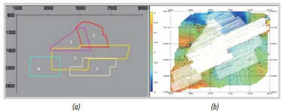
In fact, seismic data merging has been performed regularly on many foreign projects [1 - 3] and the results have been very encouraging. Figure 1 shows an example map of several overlapping surveys in India [1] subjected to the merging process.

There are several important applications of merged seismic data. The subsurface image of regions near the edges of a local survey is usually distorted from the migration due to the deficiency of input seismic data, which eventually can be compensated by another overlapped survey data [1]. The most important application is probably the ability to carry out the interpretation of structures continuously and seamlessly on the merged seismic data from one local region to another, and hence enable many geological analyses for a large area such as the structural analysis, sequence stratigraphy analysis, etc. Moreover, many attribute extraction applications can also be performed on the merged dataset such as various seismic attribute analyses, PaleoScan software, etc.

2.    Technical difficulties with merging seismic data

The process of merging seismic data is basically related to the compensation for the differences in seismic characteristics of various overlapping datasets. The variation in seismic characteristics between datasets can broadly be categorised  as coming from 2 major sources: the widely varying seismic acquisition configurations and the differences in processing technologies. We will discuss the effect of each type of variations on the seismic characteristics as follow.

    Effect of variations in acquisition schemes

Each seismic survey is usually designed with a specific goal suitable for a particular local region. Thus, different seismic surveys in nearby regions may have different acquisition parameters. We concentrate on a few important acquisition parameters.

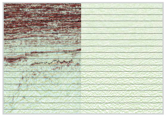Figure 2. Drastic amplitude differences between two overlapping surveys

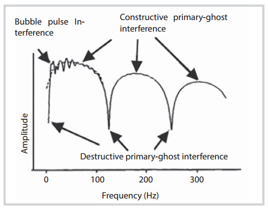Figure 3. The impact of the ghost notching frequency on the frequency content of the acquired signal [4]

The most obvious differences are due to the acquisition configuration on the survey boat such as the source configuration, including the types of the source - air gun, vibroseis, dynamite, the geometry of the source array, and the volumes of individual guns, etc. In addition, the variation in the configuration of the receiver side may include the number and length of the streamer cables, the interval of the receivers, the type of receivers such as hydrophones, velocity phones, the recording and sampling intervals, the frequency of anti-aliasing filter, etc. Those differences provide decisive impacts on the amplitude and frequency content of the acquired seismic data, the signal to noise ratio (SNR), as well as the fold density at local common middle points. Drastic amplitude differences between two overlapping surveys can be seen in Figure 2.

The frequency content differences may come from another source. Nearby surveys may have different source depths and receiver  depths  that  can affect the ghost frequencies. Typically, the ghost notch frequency is related to the source or receiver depth by the formula [4]

Where Vwater is the seismic velocity in the water medium, d is the depth of the  source  or  receiver and fnotch is the notching frequency. The effect of the ghost notch on the frequency content is illustrated   in Figure 3.

The frequency limitation by the ghost notches, in turn, will affect the signal frequency bandwidth, which will impact the seismic resolution as well as the wavelet shape. Seismic frequency content and resolution differences, as a combination of several factors, can be seen in Figure 4 where the survey on the left has a much lower frequency content and resolution, comparing with the survey on the right.

New acquisition advancements such as PGS’s GeoStreamer/GeoSource [5, 6] or CGG-Veritas’ BroadSeis [7] technologies will further widen the seismic frequency bandwidth/resolution differences comparing to the seismic data acquired from the traditional hydrophone - flat cable configuration.

The   presence   of   external    factors    such   as acquisition time (tidal change), changing weather (rough vs quiet sea for marine acquisition), changing unconsolidated layer thickness (for land acquisition) might result   in another class of problems which is the differences in phases and statics between overlapping surveys. The phase/static differences are troublesome for interpretation horizons to align from a seismic dataset to another. The effect and correction for phase/static problem is discussed further in Section 3.

Figure 4. The difference of the signal frequency bandwidth/resolution

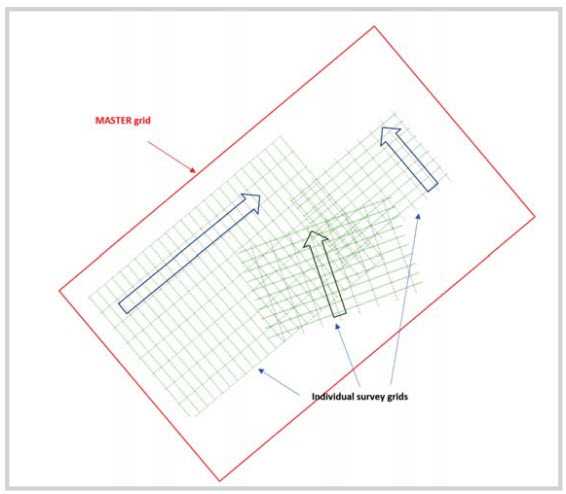Figure 5. Location map showing the Grid orientation and Master grid

A parameter that is also frequently changing from survey to survey is the acquisition azimuth/ orientation. This leads to the differences to the orientation of the migration grid (inline-crossline grid) in the post-acquisition seismic processing workflow. A typical 3 survey overlapping grid configuration is shown in Figure 5. As we can  see, each grid system has a different inline orientation, as well as different grid binning dimensions, not to mention the possible CMP- fold differences.

The discrepancy in the grid orientations eventually leads to the need to re-grid seismic datasets in to a common encompassing grid system (master grid) and re-number the inline and crossline during the seismic merging process (Section 3).

A less obvious effect of the differences in the sail-line’s direction is related to the amount of seismic illumination. For a single survey orientation, underground geological objects may have certain seismic features being illuminated better than other depending on the alignment of the object and the sail-line’s direction. This can be illustrated in Figure 6 where, as part of the survey design process at the VPI, we simulate the seismic illumination of a target horizon/ fault under different sail-line azimuths of the survey boat with other acquisition parameters kept the same. As we can see a major fault is illuminated differently under different sail-line orientation. The differences in the amount of seismic illuminations on the same geological object mean that the images of the same object on the final overlapping seismic cube may have different apparent, amplitude and image quality, which requires the amplitude conditioning before merging.
 (a)    (b)    (c)

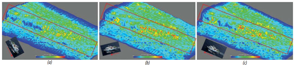Figure 6. Different seismic illumination on the same fault depending on the sail line azimuth: a. 168 degree, b. 258 degree, and c. 319 degree. Illumination by the 258 degree sail lineazimuth appears to create the clearest observation of the fault surface.

    Differences in seismic data processing routines

The differences in processing workflows from various contractors should also present some problems with merging seismic surveys. Each processing jobs may have dramatically different objectives, and technologies including:

-    Different target objects that may lie at different depth (shallow vs. deep).

-    Different technologies used in the process, such as PSTM, PSDM, and CBM, etc.

-    Different parameters used in the flows (possibly on the same dataset).

We highlight some major aspects, including phase/static, amplitudes, frequencies, and SNR, that the differences impact the merging process.

A common issue is related to the misalignment of events between two overlapping  datasets,  also   known   as the static/phase problem. Beside those originated from the survey configuration differences, the causes of the misalignment might also be traced to several processing routines:

-    The difference in velocities used in the seismic migration might lead to some events (dipping reflection planes) to be migrated to a different time/depth comparing to one processed from the other routine.

  -    The misalignment may also come from the differences between the time and depth migration, and the dipping features may not align for the PSTM and PSDM converted to time.

-    Another source of misalignments is from the different level of Q-compensation between datasets - leading to different phase shifts.

- Events at the edges of a survey is usually observed to  have  incorrect  imaging  time/depth  due to the insufficient input seismic points for the migration.

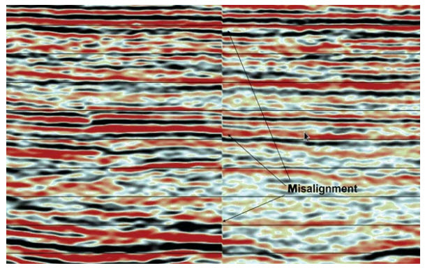Figure 7. Seismic event misalignments of two seismic survey

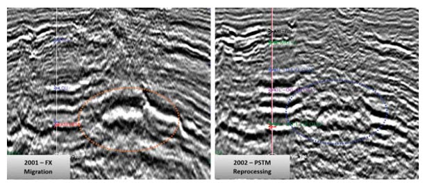Figure 8. Technology differences comparison - FX Migration vs PSTM Migration

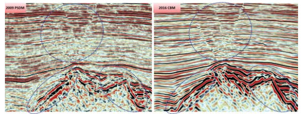Figure 9. Technology differences comparison - PSDM vs CBM

 Figure 10. Combination of the differences in seismic acquisition and processing may result in two overlapping seismic sections (left and right) with completely different appearances

Seismic event misalignments are serious because in case you are willing to align those events at a certain depth, events at other depths may still misalign.

Another discrepancy is about the amplitude between overlapping seismic data. Beside the cause from the acquisition configuration  factors (as discussed above), the variation in the seismic amplitude might be the consequence of the difference in migration apertures (each image point receives contributions from a varying number of traces). The processing flow may further contribute to it by various amplitude compensation such as the post stack time-variant scaling, Automatic Gain Control. Amplitude compensation for the absorption (Q-compensation) might be different in workflows from different processing contractors.

Thedifferences in the amount of Q-compensation might also be the source of differences in the frequency content of two overlapping surveys. Besides,  frequency  manipulation  techniques  such as spectral shaping, spectral whitening, spectral bluing, source deconvolution, and source wavelet de-ghosting, etc. might affect the frequency content between two datasets. However, for the marine data, these  drastic  frequency-altering  techniques   are not usually offered by the processing contractor to preserve the original frequency bandwidth (unless requested by the client).

An often-overlooked aspect is the merging of datasets with different SNR, which might make the final results look synthetic (a poor dataset is stitched to a good dataset). Newer computing hardware resources enable more advanced processing/ imaging algorithms that can provide seismic results with enhanced SNR and new seismic features shown up comparing to the vintage. The example shown in Figure 8 is the comparison of the seismic quality from results processed by the old FX migration in 2001 (left) and reprocessed by the PSTM algorithm in 2002, in which, the quality of PSTM seismic data is significantly improved, in terms of details (resolution) and frequency bandwidth, compared to the old (possibly obsoleted) FX migration seismic data.

Figure 9 illustrates another comparison between the old PSDM and the newer CBM processing, where many features, such as faults, top basement show up more clearly on the final CBM stack section, comparing to the vintage PSDM processing. Overlapping seismic datasets with different level of SNR will cause difficulties in matching up data, or lining-up events. A possible remedy is to perform seismic enhancement for poor quality data such as one described in a recent study from our group [8], although the results might be limited after stacking has been performed. Or better, input seismic data might be inspected before merging to select those with similar SNR.

The accumulation effect of various types of differences from the survey configuration to seismic signal processing may result in seismic sections of the overlapping region with significant different appearances such as one in Figure 10. In this case, a decision will need to be made regarding the merge border, which, in turn, will decide which part of the individual survey will remain in the merged dataset, and which part will be thrown away.

3.    Merging 3D post-stack data

The goal of the merging of 3D post-stack seismic surveys is to create a single 3D seismic cube which balances the phase and amplitude of individual stacked input seismic cubes. For geological structure and seismic attribute analysis, the results might be adequate, but certainly cannot be as good as merging pre-migration seismic data. The workflow can be summarised in 5 major processing steps as shown in Figure 11. Note that the flow chart is over-simplified and each major step can be rerun as needed.

    Regrid of seismic data

As discussed in Section 2, due to the differences in survey orientations, overlapping surveys may have different migration grids with different azimuths and different CDP spacings. Re-gridding of seismic data is essentially spatial  resampling   (i.e.   interpolation) of data by points on a common encompassing  master  grid  (Figure  5).  In our experiences, the selection of the master grid may fall into one of the two popular choices:

-    We can select the orientation of the majority of the surveys, which has  the benefit of having a smaller number of surveys to be regridded.

-    Or we can select the orientation of the master grid to be orthogonal to the major fault or features of concern.

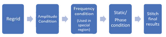Figure 11. Five major steps flowchart in merging post-stack seismic data

Various interpolation schemes exist such as bilinear interpolation, bicubic interpolation, polynomial  interpolation or spline interpolation, etc. We chose the sinc function interpolation (Whittaker- Shannon interpolation) since it is the perfect reconstruction of the original (continuous) signal according to the Shannon sampling theorem [9]. In one dimension, the interpolation takes the form of:

Where t is the continuous time/ space variable, sinc(t) = sin(πt)/(πt) and T is usually the sampling rate that gives the samples {x[n]}. From the interpolation formula,  resampling   simply   means  to choose to resample t at a different discrete rate: t = T1, 2T1,…, nT1,… In our case of spatial resampling, we use the extended 2D version of the formula. An illustration of re-gridding can be seen in Figure 12 where spatial data points that misalign with the master grid are resampled into points on the master grid (located at the centre of each new cell).

    Amplitude conditioning

Amplitude equalisation between overlapping seismic dataset usually means correcting the amplitude envelopes of one dataset to match with that of the other one. Since there could be different gain functions applied to the datasets, the amplitude correction is usually time-variant too. Figure 13 illustrates  the  results  from amplitude conditioning where the amplitude of the left section is matched to the one on the right section. Care has been taken to preserve relative amplitude so that seismic anomalies (such as Direct Hydro Carbon Indicator (DHI)) still show up correctly after amplitude conditioning, as the amplitude conditioning step only applies a constant smooth gain function (for the most part of the merging seismic cubes). As illustrated in Figure 14, a bright spot remains relatively standing out after amplitude conditioning.

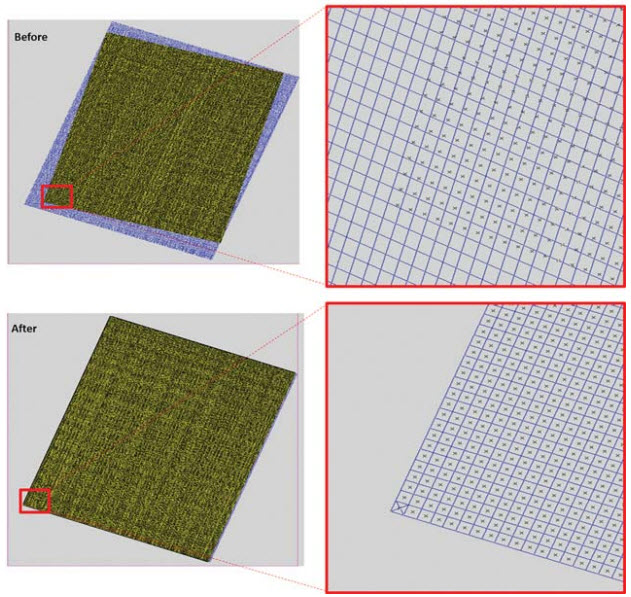Figure 12. Basemaps grid point before and after re-gridding

Figure 13. Two merging seismic sections before and after amplitude conditioning
(a)    (b)

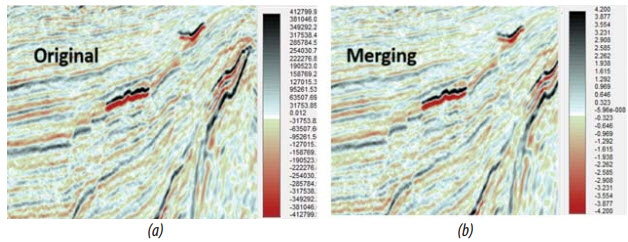Figure 14. A stack section with a bright spot before (a) and after (b) amplitude conditioning. Notice the range of amplitude of the original seismic is about -4e5 to 4e5, while the range of amplitude of the merging seismic is about -4 to 4. The bright spot has a relatively high amplitude in both cases.

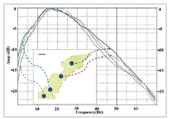   Figure 15. Average amplitude spectra from different campaigns [10]

    Frequency conditioning

Some special regions may require frequency conditioning due to the obvious differences in the frequency spectra. Thus, the frequency conditioning step aims to minimise the difference in amplitude spectra (rather than the energy in the different section). This is usually accomplished by a matching or shaping filter.

The process of frequency matching may contain an inherent conflict goal. On the one hand, we want uniform frequency bandwidth on the merged cube for the attribute analysis on the final result and the easiest way is to choose the seismic cube with the lowest frequency bandwidth as the reference and band-limit the frequency of other higher-quality cubes. Certainly, this approach will degrade the quality of some input seismic. On the other hand, we also desire to preserve as much frequency bandwidth/time resolution as possible, this implies to use the seismic cube with wider bandwidth as the reference and to perform shaping filter to enhance the frequency content of the seismic data with lower bandwidth (whitening the data). However, the result might be limited as whitening the data too much will amplify the noise. In drastic cases, a decision on a compromise frequency bandwidth might be made.

An example of performing frequency conditioning can be seen in Figure 15 [10] where the authors apply spectral whitening to smooth out frequency spectra across the datasets.

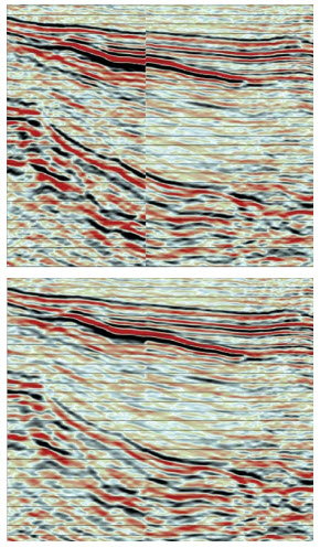Figure 16. Two merging seismic sections before and after static conditioning

The differences in the amount of Q-compensation might be another aspect that is crucial to the discrepancy in the frequency content on the deeper section. Thus, techniques such as to apply inverse Q-compensation  and  reapply  an equal amount of Q can also be carried out if information from the processing report is available.

    Static/phase conditioning

This  step  is  to  match  the  timing  and  phase  of reflection events on the overlapping region. Static/phase conditioning is crucial to merging and responsible for the smooth/seamless look of the merged cube. In the actual processing, the first thing to consider is to make sure all seismic dataset has the same polarity. This is usually obvious by inspecting major events. Optionally, performing Q-conditioning on the phase, again, might also be helpful to improve alignments of events on the deeper sections.

Static/phase conditioning, then, try to align events by the sub-sample levels. Techniques to estimate the amount of misalignment may include the time correlation or the phase spectra matching. This conditioning step then adjusts the data by static shifts and phase rotation. In our experiences, events at  the outermost edges might not be easily matched due to the migration distortion, but they are usually discarded anyway in the next step.

Figure 16 shows the effect of matching the statics from two different datasets. As we can see, major events can be matched and, hence, run continuously between the two surveys. However, the result is not perfect as some small residual artifacts of the borders remain. This is the basic limitation of performing merging  on the post-stack dataset as static/phase conditioning may not be able to match  all events from the shallow to the deeper intervals.

    Stitching final results

The last step is to merge conditioned seismic cube together. This involves border design and throwing away redundant seismic data (as shown in Figure 10). The usual added benefit is that discarded seismic is usually the data at the edges of the surveys where major distortions occur.

4.    Field data results

We present field data results from the merging process performed at EPC-VPI. Some more merging results are shown in Figure 17 where we had a seismic section before and after the merging process. As we can see, events are continuous and the whole merged section has a uniform amplitude, giving the perception of a dataset from a single seismic acquisition. The continuity of the events can be further illustrated in Figure  18  where  we took a time slice before  and  after  the merging. In this case, after merging, the border disappears and events are continuous from one side of the border to the other side.

Figure 17. Two merging seismic sections before and after merging process

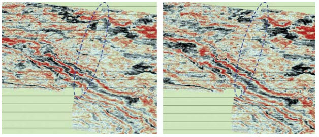Figure 18. Time slice of two merging seismic sections before and after merging process

Figure 19. RMS analysis on the merged seismic cube

We also attempted to run an RMS seismic attribute extraction from the merged seismic cube on a horizon within the Oligocene layer and the result is successful (Figure 19). The attribute map looks continuous throughout the merge borders, allowing an interpretation of features and abnormal amplitudes, although some minor artifacts from a very small overlapping area (low fold edge region) may remain.

5.    Towards 3D premigration pre-stack seismic data merging

As we have seen in Sections 3 and 4, the problem of misalignments of seismic events can be partially solved by matching phase/static from post-stack seismic cubes (Section 3.2). However, residual artifacts are frequently observed, especially on the dipping events. This problem can only be solved completely by performing a merge on the premigration pre-stack seismic data (merging before imaging) such as the studies in [10 - 13].

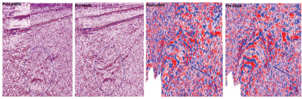
Technically, reprocessing and merging from raw data should provide a better result due to the combination of a common processing/conditioning routine, a common velocity analysis, a common migration grid, and a common migration algorithm. The advantages of the premigration- prestack merge results comparing to the post-stack merge results can be shown in Figure 20 [13] where results from the premigration-prestack seismic merging show significantly more details in the overlapping region due to the added complementary data for migration. Another illustration is shown in Figure 21 [14] from Sino Geophysical with similar observations.

Many issues that have been discussed in Section 2 may remain with premigration-prestack data merging such as the discrepancies in the shot records such as shot length, shot density, or receiver intervals, cable length which can be solved by the shot record regularisation. Another discrepancy might be related to the CDP folds (midpoint density) and require a CDP fold regularisation also. Usually, trace regularisations (such as the shot record or cdp fold regularisation) can be accomplished by the combination of the trace decimation and 5D trace interpolation.

Old post stack merging section                                                                         New prestack merging section by WEFOX

Figure 20. A comparison of post-stack and pre-stack merging [12]  

Figure 21. A comparison of post-stack and pre-stack merging [14]

Pre-stack merging of seismic data will be very  useful for pre-stack analyses such as AVO and inversion analyses, although at the cost of some serious technical difficulties. Common sense indicates that the process of merging premigration data requires huge processing resource requirements (machines and workforces), a long processing time, and a high cost. Various issues like seismic illumination and frequency bandwidth might still be present.

6.    Conclusions

3D merging of seismic surveys recorded in different acquisition processes with various acquisition geometries, orientation and processing workflows is a very intricate process. Major problems are the mismatch of amplitude, frequency bandwidth, static/phases and SNR between overlapping seismic dataset. Fundamentally  resolving each problem is necessary to achieve the goal of treatment and help the interpreters to meet the geological objectives. Our hunt for the solutions has resulted in an in-house merging workflow for the post-stack data that is relatively fast to execute and cheap to implement on the available computing hardware. Results processed at the Vietnam Petroleum Institute (VPI) show a sufficiently good merged dataset that meets the requirements of uniform amplitudes/frequencies/phases, with a seamless look of the sections/time slices, and reflection events running continuously from one area to another. Our resultant merged datasets thus look quite promising that they  could be used for seamless geological interpretation or continuous seismic attribute analysis. The limitations of the post-stack merging process including some dipping events might not be to align very well, some artifacts may remain due to small overlapping area (low fold at the edge/ migration distortion), and sometimes high-quality data may need to be downgraded to match low-quality data. Those imperfections, although looking minor, sometimes may have serious consequences in applications such as ambiguity in interpretation or producing seismic anomaly in attribute analysis, thus extreme care must be taken both during the process of performing post-stack seismic merging and during QC and recommendations, as well as during actual usage.

Looking towards the future, we would like to explore the implementation of a 3D prestack-premigration merging workflows, which should promise better, more uniform, more seamless merging results, although at a possibly much more expensive computational cost, more complex algorithms/workflows and longer run time.

References

1.    S.Basu, S.N.Dalei, D.P.Sinha. 3Dseismicdatamerging - A case history in Indian context. Geohorizons. 2008.

2.    Agus Widjiastono, Nasser Hamrbtan, Almhedwi Aljilani. Merging 3D seismic data for IR field development. North Africa Technical Conference and Exhibition, Cairo, Egypt. 14 - 17 February, 2010.

3.    M.Radovcic, S.Cumbrek, I.Nagl, T.Ruzic. 3D seismic data merging: A case study in the Croatia - Hungary border area. 6th Congress of Balkan Geophysical Society, Budapest. 3 - 6 October, 2011.

4.    Mamdouh R.Gaddalah, Ray L.Fisher. Applied seismology: A comprehensive guide to seismic theory and application. PennWell Books. 2005.

5.    PGS. Geostreamer. www.pgs.com.

6.    PGS. Geosource. www.pgs.com. 2017.

7.    CGG. Broadseis. www.cgg.com. 2017.

8.    Tạ Quang Minh, Bùi Thị Hạnh, Nguyễn Tiến Thịnh. Phân tích cấu trúc và nâng cao chất lượng tài liệu địa chấn. Tạp chí Dầu khí. 2017; 8: trang 16 - 24.

9.    Alan V.Oppenheim, Ronald W.Schafer, John R.Buck. Discrete time signal processing (2nd edition). Prentice Hall. 1999.

10.    Bera. Prestack 3D land data merging a case history from south Asian shelf India. SPG India - 11th Biennial International Conference and Exposition. 2015.

11.    Wang Lixin. The pre-stack merging imaging techniques and its applications. SEG Technical Program Expanded Abstract. 2010: p. 2870 - 2874.

12.    Jun Cai, Manhong Guo, Shuqian Dong. Merging multiple surveys before imaging. SEG San Antonio 2011 Annual Meeting. 2011.

13.    A.K.Srivastav, C.Chakravorty, K.V. Krishnan. Some issues in 3D Pre-stack merging. 8th Biennial International Conference & Exposition on Petroleum Geophysics. 2010.

14.    Sino Geophysicals Co. 3D pre-stack merging processing technology. www.sinogeo.com. 19/9/2017.