Different forms of Gassmann equation and implications for the estimation of rock properties
Summary
Three new equivalent forms of Gassmann equation are presented that are useful when the unknown parameters are the Biot- Willis coefficient, the dry bulk modulus, and/or the grain matrix bulk modulus. We apply these equations to several sets of laboratory measurements to determine the profiles of grain matrix bulk modulus and Biot-Willis coefficient as functions of applied pressure, and perform a Monte Carlo simulation to examine the effect of uncertainty and/or measurement errors on the calculated grain matrix bulk modulus and Biot-Willis coefficient. The results show that the calculated grain matrix bulk modulus is relatively constant with applied differential pressure (up to 50MPa). However, it is very sensitive to the uncertainty of dry and saturated bulk modulus values. Thus, the presented new forms of Gassmann equation can be used to effectively quantify the uncertainty of dry and saturated bulk modulus (and subsequently, the seismic velocities) in fluid identification, fluid substitution, or reservoir monitoring applications.
Key words: Gassmann equation, bulk moduli, Biot-Willis coefficient, sensitivity analysis.
1. Introduction
The Gassmann equations [1] have been used extensively in the oil and gas
industry for fluid identification and reservoir monitoring
applications, despite its various assumptions [2, 3]. The first Gassmann
equation provides the relationship between the saturated bulk
modulus of a rock and its dry frame bulk modulus, porosity, bulk
modulus of the mineral matrix, and bulk modulus of the pore-filling
fluid. Whereas, the second Gassmann equation simply states that the
shear modulus of the rock is independent of the presence of the
saturating fluid:

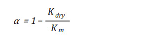
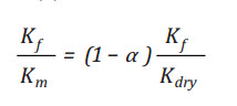
Where α is the Biot-Willis coefficient [4]:
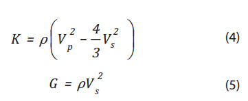
The moduli are related to the seismic velocities and density by:
Berryman [5] gave a concise derivation of Gassmann equations for an
isotropic and homogeneous medium using the quasi-static
poroelastic theory. Other forms of Equation (1) can be found in
Mavko et al. [6]. Zimmerman [7] presented an equivalent form in terms
of compressibility. However, Equation (1) is probably the most
intuitive in describing the effect of fluid presence on the bulk
modulus.
White and Castagna [8] argued that, since all input parameters for Gassmann equations carry some degrees of uncertainty, a fluid modulus inversion should be performed using a probabilistic approach. Artola and Alvarado [9] evaluated the effect of uncertainty of different input parameters and showed that the computed compressional velocity of a saturated rock is most sensitive to uncertainties in the rock bulk density and the dry bulk and shear moduli, while other parameters (porosity, the grain matrix and fluid bulk moduli) have negligible effects.
Note that the three parameters: dry frame modulus (Kdry), Biot-Willis
coefficient (α), and grain matrix bulk modulus (Km) are related by
Equation (3); in many instances they are unknown. The fluid saturated
bulk modulus (Ksat) and fluid bulk modulus (Kf) can also be unknown
(e.g. in fluid substitution problem). Asaresult, ad-hoc and empirical
correlations have been proposed to address this problem. There are many
instances Biot-Willis coefficient is assumedto be 1 due to the lack of a
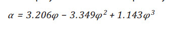
better estimate. For sandstone at high differential pressure
(40MPa), Han and Batzle [10] proposed α to be a polynomial function of
porosity:
In this study, we present 3 new equivalent forms of Gassmann equation
that are useful for different scenarios of available data. We apply
these equations to several sets of laboratory measurements. A
stochastic simulation is performed to examine the effect of uncertainty
and/ or measurement errors on calculated grain matrix bulk modulus
and Biot-Willis coefficient.
2. The new equivalent Gassmann equations
When (K , K , K , and φ) are known
This is generally the case for laboratory measurements on dry and wet
rock samples (e.g. dry and brine saturated acoustic velocities are
measured as functions of differential pressure along with rock
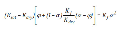
porosity). In this case we can rewrite Equation (1) as a function of
Biot-Willis coefficient α (see Appendix A for a detailed derivation):
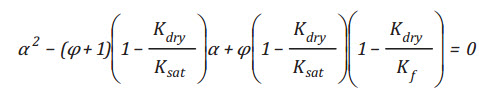
Equation (7) is a quadratic equation A2 + B + C = 0, where all coefficients can be readily calculated.
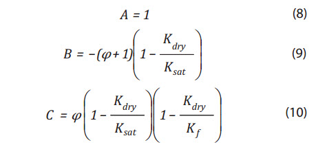
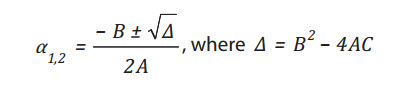
This simple quadratic equation has two solutions:
 (11)
(11)
However, Berryman and Milton(11) showed that α is physically bounded
between 0 and 1. Equations (9) and (10) show that B is negative since
Kdry < Ksat, and C is also negative since Kf < Kdry for
consolidated rocks. This means
∆ = B2 – 4AC> B2 and thus, 1=…. Is the only.
Therefore, instead of having two non-linear equations for two unknowns
(α and Km), we reduce the problem to one simple quadratic equation,
Equation (7), that always gives one physically realistic solution.
This provides an independent methodology to calculate the grainmatrixbul kmodulusofarockfrom SCAL laboratory acoustic measurements of dry and saturated rock samples. Traditionally, the grain matrix bulk moduli are estimated from averages of the rock mineralogical composition (e.g. Voigt-Reuss-Hill average or Hashin- Shtrikman bounds). These bounds may carry large uncertainties since many minerals, especially clays, have a high variance in their bulk modulus values depending the measurement conditions [12, 13]. We can further postulate that: (a) the grain matrix calculated from Gassmann equation (using Equations (8) to (12)) must lie between the two bounds obtained from mixture theory, and (b) the calculated grain matrix values are insensitive to the first order to the applied pressure. Equations (7) to (11) can also be used to verify the applicability of existing estimate Biot-Willis coefficient) for different rocks.
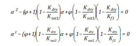
2.2. When (Ksat1, Ksat2, Kf1k Kf2, and ɸ)are known
This case can be encountered in the field. The same rock can be fully saturated with brine in one well; or it can have verying saturation in the same well. Acousstic logs, and density- porosity logs are available. In this case, K , K , and α are unknown in a system of three non-linear equations (two Equation (1) for two different saturation fluids and Equation (3)). Starting from Equation (7) instead, we end up with (see Appendix B for detaild derivations)
 (12)
(12)
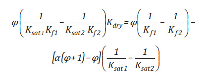 (13)
(13)
We can write Equation (13) in a more convenient form for numerical calculations:
possible solution since α2 is negative.
The corresponding grain matrix bulk modulus then can be calculated from Equation (3):
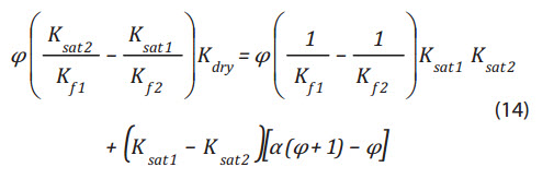
Kdry, α, and Km can now be calculated very quickly using a simple iteration using Equation (14) and Equation (7) as follows:
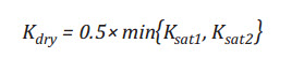
- Step 1: Make an initial guess, for example:
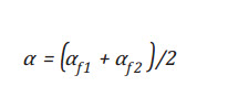
- Step 2: Use guessed Kdry value in Equation (7) to find two Biot-Willis coefficients αf1 and αf2 (for two saturations):
- Step 3: Take the average for a new Biot –Wills coefficient
- Step 4: Use this new α in Equation (14) to find new Kdry.
- Step 5: Repeat steps 2 to 4 until Kdry converges:

- Step 6: Use Equations (7) and (12) to find corresponding α and Km.
Note that we have assumed there are no softening or hardening effects caused by the saturating fluids on the grain bulk modulus (Km is constant). The secondassumption is that the rock dry frame is stiffer than both fluids, Kdry > max { Kf 1, Kf 2 }, so that Equation (7) still gives only one positive (physically realistic) root. This assumption is generally valid for consolidated sedimentary rocks.
2.3. When (Km, Ksat, Kf, and φ) are known
In this case Kdry and α are unknown. An instance for this case is that
fluid data, fluid saturation, acoustic log (Vp, Vs) and density-porosity
log are available while Km is estimated from the mineralogical
composition of the rock (FTIR, XRD, thin section of rock cuttings, or
mineralogy log). The Biot-Willis coefficient can be estimated directly
from the following equivalent Gassmann equation (see Appendix C for
detailed derivations):
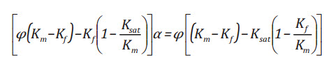 (15)
(15)
And applying this α to Equation (3) gives Kdry. This is equivalent to the Kdry solution of Zhu and McMechan [14].
3. Numerical applications
Han and Batzle’s sandstone data
We applied Equation (7) to the pressure dependent sandstone sample published by Han and Batzle [10] (Figure using the density relaρtionshρip:
 (16)
(16)
The calculated Biot-Willis coefficient and grain matrix modulus as
functions of pressure are plotted in Figure 1. The relatively constant
value of the grain bulk modulus (39GPa) as a function of pressure is a
good indicator that Gassmann equation is applicable for this rock. The
variation of grain bulk modulus at low confining pressure (< 10MPa)
is possibly due to higher uncertainty in input values (i.e. higher
noise-to-signal ratio from velocity signals).
The Biot-Willis coefficient profile is remarkably similar to the result measured on a 26% porosity Boise sandstone sample by Fatt [15]. Note that Gassmann equation gave a higher value (0.73 at 40MPa) than Han and Batzle’s Equation (6) (0.63).
Coyner’s limestone data
We employed the iteration procedure using Equations (7) to (14) on
water and benzene saturated Bedford limestone sample published by
Coyner [16] (Figure 2). In his experiment at room temperature, the
fluid pore pressure in both saturation cases was maintained at 10MPa.
The porosity of the rock is 11.9%. The shear modulus profile is
almost identical for all vacuum dry, water saturated, and benzene
saturated cases, suggesting
The back-calculated dry bulk modulus is also plotted (as a dashed line)
against the various measured moduli in Figure 2. The profile is
consistently higher than the measured vacuum dry bulk modulus profile by
approximately 2.5GPa (or 5 - 9%). This is another evidence supporting
the argument that the vacuum dry measured bulk modulus is too dry and
should not be used in Gassmann equation [6, 17]. We could have applied
the measured vacuum dry and either water- or benzene-saturated moduli
values on Equation (7), but that approach would give unrealistically
high grain matrix bulk modulus.
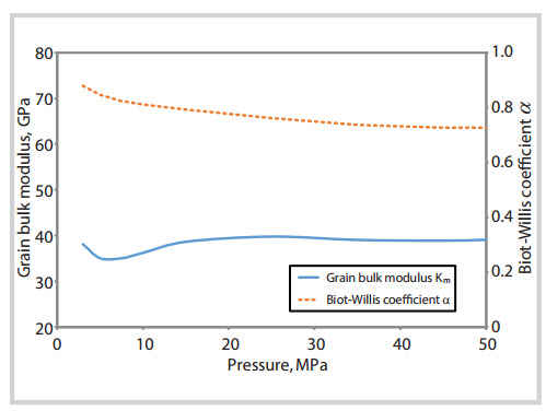 |
Figure 1. Grain bulk modulus and Biot-Willis coefficient of a sandstone
sample as a func- tion of pressure calculated from its dry and brine
saturated moduli [10] using Gassmann equation.
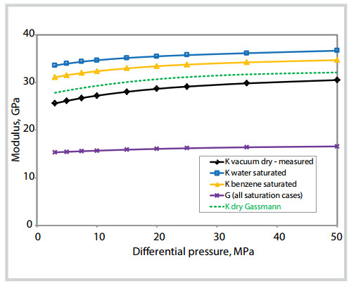 |
Figure 2. Bulk and shear moduli as a function of differential pressure
for Bedford lime- stone [6]. The dashed line is the dry bulk modulus
calculated from Gassmann equation, consistently higher than the vacuum
dry measured data.
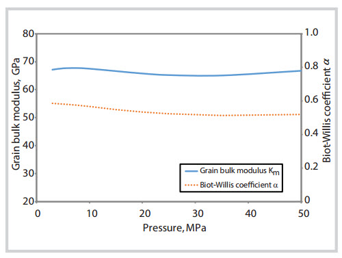 |
Figure 3. Calculated grain matrix bulk modulus and Biot-Willis coefficient of Bedford limestone sample as a function of pressure using Gassmann equation from its water - and benzene - saturated moduli [16].
The grain matrix bulk modulus and Biot-Willis coefficient profiles obtained from the rock water- and benzene-saturated moduli are shown in Figure 3. While the grain matrix bulk modulus is similar to Coyner’s reported value of 65GPa, the back-calculated Biot-Willis coefficient profile decreases from 0.6 to 0.53, significantly lower than the commonly assumed value of 1 while significantly higher than the estimated value of 0.34 obtained from Han and Batzle’s 2004 correlation.
Effects of input data errors on calculated grain bulk modulus
Measured values always have some associated errors. Velocities, especially shear wave velocities may carry significant uncertainties. We would like to determine the effects of uncertainties from porosity, Kdry, Ksat, and Kf to the uncertainty of the predicted Km. Since the relationship in Equation (7) is not linear, a Monte Carlo (stochastic) simulation was used.
Table 1 summarises the input parameter values [18] and their
estimated ranges of uncertainties. The rock sample is a Berea
sandstone sample with Voigt- Reuss-Hill average grain bulk modulus of
39.6GPa from its mineralogical composition. All parameters were assumed
to have a normal distribution with means being the measured values and
the errors represent the 95% confidence interval. Thus, the relative
error (uncertainty) of each parameter is defined as:
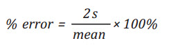 (17)
(17)
Where s is the standard deviation of the parameter’s sample.
For each set of perturbed errors, 10,000 sets of (porosity, dry bulk modulus, wet bulk modulus, and fluid modulus) values were generated to compute 10,000 grain bulk moduli, which are then analysed for the mean value and standard deviation.
In our base case, porosity is assigned a 1% error, Kdry and Ksat are
each assigned a 3% error, and Kf carries a 10% uncertainty. The
resulting Km is also a Gaussian distribution with a mean of 44.6GPa and a
standard deviation of 3.45GPa. The 95% confidence interval is,
therefore, from 37.7GPa to 51.5GPa (or 16% error). The Biot-Willis
coefficient α is also a Gaussian distribution with a mean of 0.62 and a
standard deviation of 0.03. The 95% confidence interval is from 0.56 to
0.68 (or 10% error).
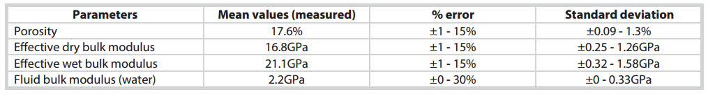 |
Table 1. Mean (measured) values of a Berea sandstone sample [18] and ranges of uncertainties used in Monte Carlo simulations
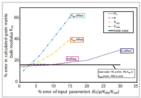 |
Figure 4. The uncertainty of the computed grain matrix bulk modulus Kmusing Gassmann equation as functions of percent error in one input parameter (Kf, α, Kdry, or Ksat), while the remaining input parameters carry the same errors as the base case. Errors from Ksat and Kdry have the largest impacts on the uncertainty of calculated Km. Porosity and fluid bulk modulus, on the other hand, show negligible effects.
Figure 4 shows the uncertainty of the computed grain matrix bulk modulus Km as functions of percent error in one input parameter (K , φ, K , or K ), while the remaining input parameters carry the same uncertainties as of the base case. Errors from Ksat and Kdry have the largest effects on the uncertainty of Km. Minus errors in Kdry and Ksat (even within laboratory measurement standard) can result in a large error in the estimated value of Km. Porosity and fluid bulk modulus, on the other hand, show negligible influence. This result is not surprising, as Kf, φ and Km should be uncorrelated parameters.
4. Conclusions
Three equivalent forms of Gassmann equation were presented that can be useful for the determination of Biot-Willis coefficient, dry bulk modulus, and/or grain matrix bulk modulus of a rock. We demonstrated the applicability of these equations using several sets of published laboratory measurements and the implications of the results for other estimations of rock properties. Astochastic simulation was also performed to examine the effect of uncertainty and/or measurement errors on calculated grain matrix bulk modulus. The results showed that the calculated grain matrix bulk modulus is relatively constant with applied differential pressure (up to 50MPa) for sedimentary rocks. However, the estimation is very sensitive to the uncertainty of dry and saturated bulk modulus values. Our new forms of Gassmann equation can be used to effectively quantify the uncertainty of dry and saturated bulk modulus (and subsequently, the seismic velocities) in fluid identification, fluid substitution, or reservoir monitoring applications.
NOMENCLATURE
K: bulk modulus (GPa or psi)
Ksat: saturated bulk modulus (GPa or psi)
Kdry: dry (frame) bulk modulus (GPa or psi) Km: grain (matrix) bulk modulus (GPa or psi) Kf: fluid bulk modulus (GPa or psi)
G: shear modulus (GPa or psi)
Gsat: saturated shear modulus (GPa or psi)
Gdry: dry (frame) shear modulus (GPa or psi)
α: Biot-Willis coefficient (dimensionless)
φ: porosity (dimensionless)
ƿ: density (g/cc)
Vp: compressional wave velocity (km/s)
Vs: shear wave velocity (km/s)
APPENDIX A: Derivation of Equation (7)
From Equation (3) we can write:
 (A.1)
(A.1)
Rewriting Equation (1) as a function of α gives:
 (A2)
(A2)
(A3)
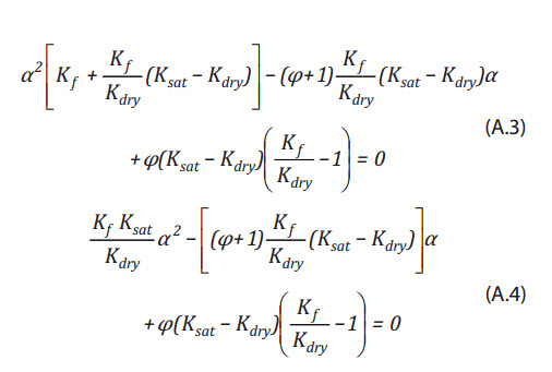
Multipplying both side with

which is Equation (7).
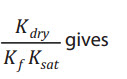
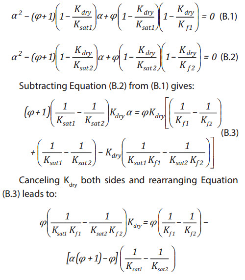
APPENDIX B: Derivation of Equation (13)
If the same rock is subjected to two different saturation fluids, then we have two equations in the form of Equation (7):
equation and rearrange Equation (1) as a function of α, the Biot-Willis coefficient only:

which is Equation (15).
APPENDIX C: Derivation of Equation (15)
If Km value can be obtained (e.g using mixture theory), then one can substitute K = (1 − α) K into Gassmann sandstones. Elsevier Science. 1991.
References
1. Fritz Gassmann. Uber die Elastizität Poröser Medien.
Vierteljahrschrift der Naturforschenden Gesellschaftin Zürich. 1951; 96:
p. 1 - 23.
2. Tad M.Smith, Carl H.Sondergeld, Chandra S.Rai. Gassmannfluid substitution. A tutorial. Geophysics. 2003; 68(2): p. 430 - 440.
3. Ludmila Adam, Michael Batzle, Ivar Brevik.Gassmannfluid substitution and shear modulus variabilityin Geophysics. 2006; 71(6): p. F173 - F183.
4.Murice Anthony Biot, David G.Willis. The elastic coefficients of the theory of consolidation. Journal of Applied Machanic. 1957; 24: p.594-601.
5. James G.Berryman. Origin of Gassmann’s equations. Geophysics. 1999; 64(5): p. 1627 - 1629.
6. Gary Mavko, Tapan Mukerji, Jack Dvorkin. The rock physics handbook: Tools for seismic analysis in porous media. Cambridge University Press, Cambridge. 1998.
7. Robert W.Zimmerman. Compressibility of which is Equation (13). Equation (14) then can be readily obtained by multiplying both sides by (Ksat1 × Ksat2).
8. Luther White, John Castagna. Stochastic fluid modulus inversion. Geophysics. 2002; 67(6): p. 1835 - 1843.
9. Fredy A.V.Artola, Vladimir Alvarado. Sensitivity analysis of Gassmann's fluid substitution equations: Some implications in feasibility studies of time-lapse seismic reservoir monitoring. Jounal of Applied Geophysics. 2006; 59(1): p. 47-62.
10. De-Hua Han, Michael L.Batzle. Gassmann’s equation and fluid-saturation effects on seismic velocities. Geophysics. 2004; 69(2): p. 398 - 405.
11. James G.Berryman, Graeme W.Milton. Exact results for generalized Gassmann’s equations in composite porous media with two constituents. Geophysics. 1991; 56: p. 1950 - 1960.
12. Keith W.Katahara. Clay mineral elastic properties. SEG Technical Program Expanded Abstracts. 1996: p. 1691 - 1694.
13. Zhijing Jee Wang, Hui Wang, Michael E.Cates. Elastic properties of solid clays. SEG Technical Program Expanded Abstracts. 1998: p. 1045 - 1048.
14. Xianhuai Zhu, George A.McMechan. Direct estimation of the bulk modulu softheframeinfluidsaturated elastic medium by Biot theory. SEG Technical Program Expanded Abstracts. 1990: p. 787 - 790.
15. I.Fatt. The Biot-Willis elastic coefficients for a sandstone. Journal of Applied Mechanics. 1959; 26: p. 296 - 297.
16. Karl B.Coyner. Effects of stress, pore pressure, and pore fluids on bulk strain, velocity, and permeability in rocks. Ph.D. dissertation, Massachusetts Institute of Technology, Cambridge, Massachusetts. 1984.
17. Virginia A.Clark, Bernhard R.Tittmann, Terry W.Spencer. Effect of volatiles on attenuation (Q-1) and velocity in sedimentary rocks. Journal of Geophysical Research. 1980; 85(B10): p. 5190 - 5198.
18. Tran Trung Dung, Chandra S.Rai, Carl H.Sondergeld. Changes in crack aspect-ratio concentration from heat treatment: A comparison between velocity inversion and experimental data. Geophysics. 2008; 73(4): p. E123 - E132.