Summary

Deep learning (DL) neural network analysis is the latest development from the Artificial Neural Network (ANN) and it is being used more and more in petroleum engineering. In this study, the way to develop a new DL model for well log analysis was attempted and successfully implemented using well log data from a location in the Cuu Long basin, Vietnam. Three sets of analyses were conducted, i.e., the first analysis set with a single hidden layer ANN model, the second analysis set with multiple hidden layer ANN model and the third with a DL neural network model. The DL-predicted porosity for a fractured granite basement reservoir of an oil field in the Cuu Long basin was found in the range from 0.0 to 0.082, showing a good match with the conventionally-calculated values. The final deep learning model consists of 5-input layers of gamma ray (GR), deep resistivity (LLD), sonic (DT), density (RHOB) and neutron porosity (NPHI), having 5 hidden neuron layers with 14 neurons per layer. It is worth noting that the transfer function of the rectified linear unit (ReLU), typical for a deep learning analysis, was implemented to replace the common sigmoidal transfer function, ensuring the successful application of DL model. Last but not least, the problem of vanishing gradient specific for a DL neural network model was also explained in details in this paper.

Key words: Deep Learning (DL), Artificial Neural Network (ANN), fracture porosity, well log analysis, fractured granite basement, Cuu Long basin.

1.    Introduction

The concept of soft computing was first put forward by a paper named “Possibility theory and soft data analysis” [1]. While hard computing needs a precisely defined analytical model, soft computing is tolerant of uncertainty, imprecision, approximation and partial truth. This is a method designed to model and solve real world problems, which cannot be modelled mathematically. The concept of soft computing was  designed based on the concept of human brain functioning.

Soft computing consists of few principal components as listed below [2]:

-    Fuzzy logic;

-    Evolutionary computation;

-    Neural computing;

-    Probabilistic reasoning.

ANN has been developed to simulate the neural structure and activity of the human brain. Deep learning (DL) is a complex version of artificial neural networks. It is now widely used in image recognition, voice processing and language translation.

Artificial neural networks are used to build a connection between input and output data that helps predict the outputs of a set of new inputs (Figure 1).

Application of deep learning in petrophysics is still in its infancy stage. Classic neural networks commonly use one hidden layer, whereas deep learning uses multiple hidden layers. The use of multiple hidden layers can cause a phenomenon called vanishing gradient problem. Deep learning network is obtained by eliminating this problem.

Conventional methods  to  estimate  the   primary   (or intergranular) porosity of clastic reservoirs are not helpful to estimate the fracture porosity. Therefore, petrophysicists keep trying to find new techniques for fracture porosity estimation.

Kohli and Arora [3] did a research on application of artificial neural networks for well log analysis. They used data from three wells including gamma ray (GR), resistivity (RES), density (RHOB), neutron porosity logs (NPHI) as the input data and the core permeability as the target data for the ANN analysis. Kohli and Arora also concluded that ANN could be relied upon for determination of characteristics even in areas where cores are not available. The estimation was completely data-driven and did not require any prior assumption. More than that the method was cost effective since it did not require labourious core analysis.

Korjani et al. [4] carried out a research on a new approach of reservoir characterisation using deep  learning neural networks for Kern River field located in San Joaquin valley, California. The field consists of nine production formations. The study was carried out using data from 473 wells. Well log data such as deep resistivity, medium resistivity, and neutron porosity were used as input parameters. The authors came to conclude that deep learning is an effective method for characterisation of a reservoir with large volumes of data.

Guler et al. [5] carried out a study on predicting relative permeability of a hydrocarbon reservoir using an artificial neural network. First, they found what should be the key input data, i.e., common fluid and rock properties were selected as the input data set. In addition, when selecting these data, they focused on parameters that could be measured in laboratories and/or easily obtained from literature. Based on the results of their study, the authors concluded that with the increase in the number of property-based input parameters, the efficiency of the ANN model was enhanced.

In the last decade, researchers from the Asian Institute of Technology (AIT) had conducted a number of studies  on application of soft computing in well  log  analysis  using fuzzy logic and neural computing [6]. For example, Witthayapradit [7] carried out a research on an integrated petrophysical study using well logging data for enhancing a gas field in the Gulf of Thailand. He originally used gamma ray (GR), deep resistivity (LLD), density (RHOB), neutron porosity (NPHI) and sonic log (DT) as the input parameters to predict porosity and permeability. Target values were obtained from core analysis data. Optimal porosity prediction was given by an ANN model with one hidden layer having 15 neurons. Optimal permeability prediction was found by an ANN model having one hidden layer with 9 neurons. Nakapraves [8] carried out a research, using two ANN models to predict reservoir porosity for a clastic oil field in the northern Pattani basin, Gulf of Thailand. In the first model, GR, LLD, RHOB, NPHI and DT logs were used as input data. In the second model, the seismic attributes such as dip, azimuth, instantaneous phase and relative acoustic impedance were used as input parameters. Core porosity was used as the target values in both models. It was found that the ANN model trained using seismic attributes gave far better results than the model trained using well log data. Foongthoncharoen [9] did a research on prediction of permeability and water saturation using neuron networks and fuzzy logic for a clastic reservoir in the Gulf of Thailand. Permeability and water saturation were predicted for two wells. Well log data of gamma ray, deep resistivity, medium resistivity, density and neutron porosity were used as input parameters. Core permeability and water saturation calculated by using Indonesian model were used as target values. Between the two models of ANN and fuzzy logic, the latter one gave better results. Sakulluangaram [10] did a research on petrophysical modelling for the Miocene Sand in the South Fang basin, northern Thailand, where he predicted porosity distribution of a well (well A) using the data from a nearby well (well B). GR, RHOB, NPHI and DT logs were used as the input parameters. Porosity values predicted were similar to the porosity obtained from well logs. Thanh [11] did an ANN prediction of porosity using the integrated well log and seismic attribute data including reflection amplitude, instantaneous amplitude, its 1st and 2nd derivative, as well as instantaneous phase, frequency, dominant frequency and reflectivity as  the  input  for an ANN model. The final porosity output determined using a Bayesian Regulation training algorithm gave the best match with the highest R-value of 0.86. Kano [12] predicted porosity for a fractured basement reservoir with well log data from two wells using a conventional method proposed by Elkewidy and Tiab [13] and five soft computing techniques, including ANN, Fuzzy Inference System with Mamdani’s style, Fuzzy Inference System with Sugeno’s style, Fuzzy Subtractive Clustering and Adaptive Neuro-Fuzzy Inference System (ANFIS). These Artificial Neural Networks gave the best prediction. Duangngern

[14]    did a fuzzy analysis to predict the effective porosity of a clastic reservoir in the Pattani basin, Thailand. He applied various Fuzzy logic techniques, using well logging and core data of two wells. Among three fuzzy techniques used, the fuzzy subtractive clustering was found the best for prediction of effective porosity with low value of root mean square error, high value of R2 and R-value. Wang

[15]    carried out a research on ANN-based prediction of fractured rock mass hydraulic conductivity for the Frieda River copper-gold mine in Papua New Guinea. In this study, the backpropagation neural network (BPNN) was trained to successfully map the relationship between indicative rock parameters and hydraulic conductivity using a variety of rock data sets collected in the site investigation of a feasibility study for the study mine. Input data were selected for ANN analysis included lithology, weathering, fracturing, unconfined compressive strength (UCS), defect angle and rock quality designation (RQD). Different numbers of input parameters (4, 5 and 6) were used to build the ANN model. Wang [15] also investigated the effect of various transfer functions on the ANN model by using log-sigmoid, tan-sigmoid and purelin.

2.    Vanishing gradient problem of multiple deep learning neural network analysis

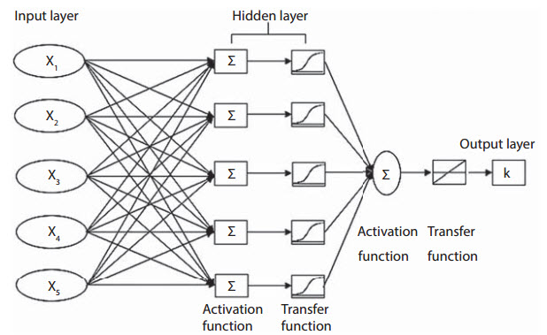 Figure 1: Architecture ò an ANN

Figure 2. Simple multi-layer ANN model after introducing the cost function

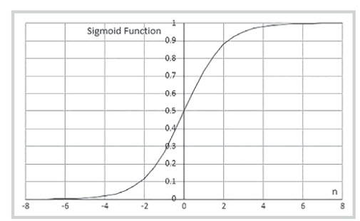Figure 3. Graphical representation of sigmoid function [12]

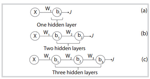Figure 4. Different ANN modes: (a) ANN model with one hidden layer; (b) ANN model with two hidden layers; and (c) ANN model with three hidden layers

Deep learning is a machine learning algorithm which could learn complex functions. The learning process of deep learning algorithm filters important information from raw data in a systematic way.

Deep learning architecture consists of multiple hidden layers comparing to shallow neural networks that used to have one hidden layer. With multiple hidden layers, a problem called vanishing gradient occurs during back propagation, thus any deep learning network should be able to overcome this problem.

Deep learning networks, like other ANN’s, have a predicted and an expected (target) value. The intention of learning is to make the difference between the target and the expected values as small  as  possible (which we assign as the goal). To understand how vanishing gradient occurs, a simple deep neural network to predict a cost function with single neuron in each hidden layer is considered as shown in Figure 2, where x is the input, W1, W2, W3, and W4 are the weights, b1, b2, b3, and b4 are the biases, and J is the cost function of the network.

In Figure 3, J represents the cost function, which    is a function of the difference between predicted and expected values. Artificial neural networks usually make use of the following sigmoid function as the activation function or transfer function:

Where:
S(n): The sigmoid function n is variable

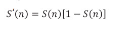
One of the reasons for popular use of the sigmoid function is that its derivative can be easily calculated by the very value of sigmoid function as follows:

  (2)
Where:

S' (n): The derivative of sigmoid function

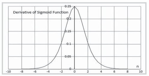Figure 5. Graphical representation of the derivative of sigmoid function [12]

Vanishing gradient problem
The derivative of sigmoidal function is plotted in Figure 5 which shows it lies between 0 and 0.25.
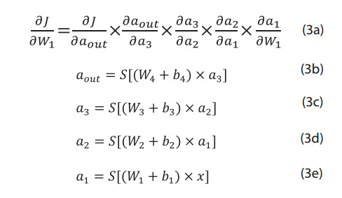
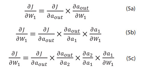
By the chain rule, the derivative of the error (J) with respect to the first weight (W1), can be written as:
Where:
 
Where:

a out: Output of the ANN network;

a1: Output from the first hidden layer;

a2: Output from the second hidden layer;

a3: Output from the third hidden layer;

W1: Weights of the input layer;

W2: Weights of the first hidden layer;

W3: Weights of the second hidden layer;

W4: Weights of the third hidden layer;

x: Inputs of the ANN; S: Sigmoid function.

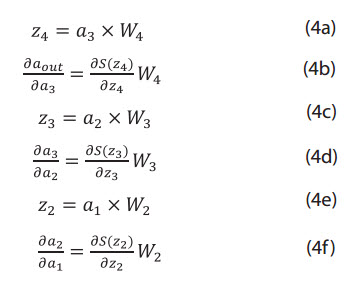
Considering the following derivative components in Equation 3a

In Figure 2, by denoting the inputs to the 4th, 3rd, 2nd hidden layers as z4, z3, z2 respectively, one can write the following relationships:

 Where:

S: Sigmoid function;

z2: Input to the second hidden layer;

z3: Input to the third hidden layer;

  z4: Input to the output layer.

The maximum value that the derivative of the  sigmoid function can take is 0.25 (and the minimum is 0). The weights are selected based on Gaussian distribution, thus the value of weights always lies between -1 and 1.

When the values of each  derivative  are  multiplied  by each other, the resultant will give a small value less than 1. Imagine if the number of hidden layers increased, becoming deeper and deeper, the number of derivative terms will increase as well as the number of terms to be multiplied (Equations 5a-c), making the resulting value of smaller and smaller. This shows how early layers learn slower with the increase of the number of hidden layers. A similar approach can be implemented to show that latter layers learn faster by obtaining the derivation of cost function with respect to W3.

Vanishing gradient occurs because of using the sigmoid function. To overcome the problem, an alternative activation function known as rectified linear unit (ReLU) was introduced in deep learning.

3.    Methodology of this study

The well log data were collected from a well drilled into a fractured granite basement (FGB) reservoir in an oil field of Cuu Long basin for a depth range from 2,525m to 3,015m including gamma ray (GR), deep resistivity (LLD), shallow resistivity (LLS), interval transit time (DT), bulk density (RHOB), neutron porosity (NPHI), photoelectric factor (PEF), and caliper (CAL). Figure 6 shows the general workflow of this study.

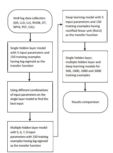Figure 6. Flow chart of the study’s methodology

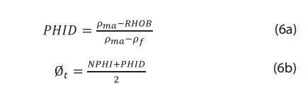
The total and fracture porosity for the target data set was calculated using the approach suggested by Elkewidy and Tiab [13] as shown in Equations 6a and 6b below. Matrix density was assumed as 2.71g/cc since formation density and porosity were measured in limestone scale.

Where:

Øt: Total porosity (fraction);

NPHI : Neutron porosity (fraction);

PHID: Porosity calculated from bulk density (fraction);

RHOB: Bulk density of formation (g/cc);

ρma: Matrix density, assumed to be 2.71g/cc (since measured in limestone scale);

ρf: Fluid density, assumed to be 1g/cc (water).

An equation to calculate fracture porosity of a fractured reservoir can be derived by using the following steps:

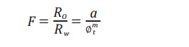
The formation factor (F):
(7a)

and fracture intensity index (FII):
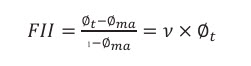 (7b)

By rearranging Equation 7b, the matrix porosity is:
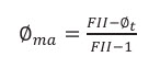(7c)

As fracture porosity (øf) is: 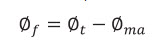(7d)

by replacing øm in 7d with 7c, one has:
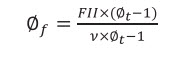(7e)

For a double porosity fractured reservoir with 100% formation fluid saturation one can write: 7 (f)
(7f)
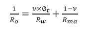
Where Rma is the resistivity of 100% fluid saturated matrix and Ro is the resistivity of the total system (matrix voids + fracture voids) being 100% fluid saturated.

Rearranging Equation 7f and combining with Equation 7a one gets:

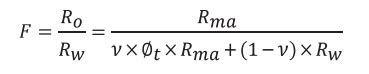(7g)

 (7h)
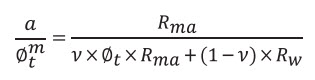
Assuming a = 1 and with further rearranging Equation 7h one has:

  (7i)
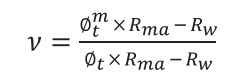
 In case, one can neglect water resistivity (Rw) in Equation 7i since Rma >> Rw, the porosity partitioning coefficient can be expressed as:

(7j)

By replacing 7j with 7b one has:  (7 k)

(7k)
Further replacing Equation 7k with 7c and 7e one gets:   

(7l)

Hence the target (fracture porosity) will be:

(7m)

Where:

Øf: Fracture porosity (fraction);

Øma: Matrix porosity (fraction);

m: Cementation exponent.

Partitioning coefficient (ν), matrix porosity (Øma), and fracture porosity (Øf) are calculated by Equations 7j, 7l and 7m, respectively [13]:

Data from the depth interval of 2,515- 3,015m were selected and analysed for each 0.125m interval. Three conducted analyses are summarised in Table 1 and named as I, II and III. In analysis I, only five inputs out of the eight well log parameters were investigated. A total of 16 combinations, denoted as MI1 to 16 (Table 1), will be done to find out the best combination of 5.

Based on the criteria proposed by Guller et al. [5], the combination of five selected input parameters having the least prediction error at 150 training examples will be further tested for training examples of 500; 1,000; 2,000 and 3,000, respectively. In analysis II, with multiple hidden layer ANN model,  the first issue to be studied is what would happen if one uses more than 5 input parameters, for example 6, 7 and 8 input parameters. After that, the effect of the number of training examples will be also investigated. Inanalysis III, adeeplearning model will be developed from the best multiple hidden layer model found in Analysis II by replacing the sigmoidal transfer functions with the rectified linear units (RELU). The deep learning (DL) models will also be investigated for various number of hidden layers as well as number of training examples, i.e., 50; 500; 1,000; 2,000 and 3,000.

The fracture porosity values predicted by all of the ANN and DL models in analyses I, II and III will be plotted and compared between them as well with the fracture porosity values calculated by the method proposed by Elkewidy and Tiab [13] as explained above in detail (Equation 7f).

4.    Results and discussion

In Analysis I, ANN models with a single hidden layer were analysed. Firstly, 16 models numbered from MI1 to MI16 (Table 1) were tested with 150 training examples to find out the best combination of five input parameters out of 8 well log data used (GR, LLD, LLS, DT, RHOB, NPHI, PEF and CAL). It was found that the model with the basic 5-input sets (GR, LLD, RHOB, NPHI and DT), 12 neurons of the hidden layer and running for 150 training examples (Figure 7) gave the best prediction of fracture porosity with the least prediction error (Table 2). Four more models in Analysis        I, numbered from MI17 to 20 (Table 1), were tested with the number of training examples increased from 150 to 500; 1,000; 2,000 and 3,000 respectively, and with different number of neurons in the hidden layer. However, prediction of fracture porosity did not improve (Figure 7).

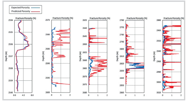Figure 7. Fracture porosity calculated by single hidden layer ANN models, Analysis I, with 150; 500; 1,000; 2,000 and 3,000 training examples as seen from left to right

Figure 8. Fracture porosity calculated by multiple hidden layer ANN models, Analysis II, with 150; 500; 1,000; 2,000 and 3,000 training examples as seen from left to right

In Analysis II, various multiple hidden layer ANN models (Table 1) were tested to see if the prediction of fracture porosity would increase with the increasing number of hidden layers using the basic set of five input parameters as found in Analysis I. It was found that model MII1    with 4 hidden layers and 12 neurons per layer gave the least prediction error of 16.46% after 150 training examples. When the number of training examples increased from 150 to 500; 1,000; 2,000 and 3,000 respectively, the prediction of fracture porosity was not improved either (Figure 8).

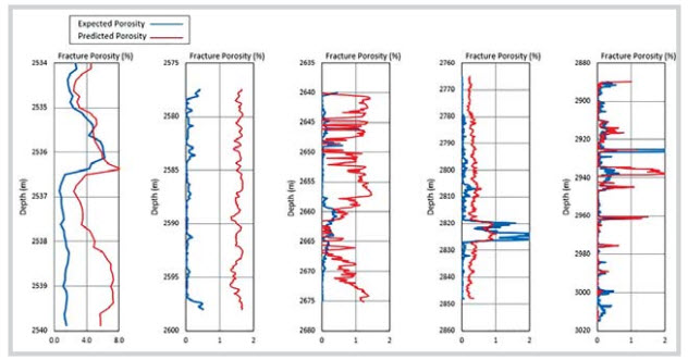Figure 9. Fracture porosity calculated by deep learning models, Analysis III, with 150; 500; 1,000; 2,000 and 3,000 training examples

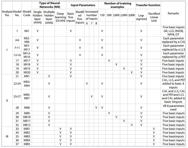Table 1. Summary of ANN and deep learning models in this study

In Analysis III, deep learning models were developed using the ReLU transfer function and tested. A total of five models numbered from MIII1 - MIII5 as seen in Table 1 were run with the basic set  of five input parameters (GR, LLD, RHOB, NPHI and DT) and with training examples of 150; 500; 1,000; 2,000 and 3,000. The

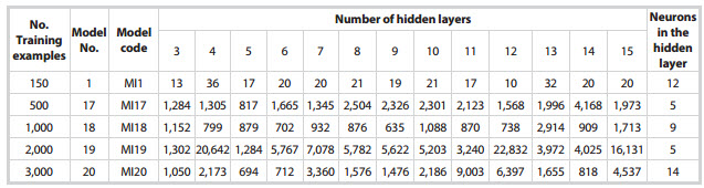Table 2. Average prediction error for different number of neurons in single hidden layer ANN models, Analysis I, with 150; 500; 1,000; 2,000 and 3,000 training examples

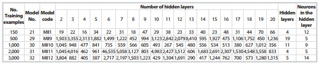Table 3. Average prediction error for different number of neurons in multiple hidden layer ANN models, Analysis II, with 150; 500; 1,000; 2,000 and 3,000 training examples

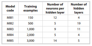Table 4. Average prediction error for different number of neurons in deep learning model with 150; 500; 1,000; 2,000 and 3,000 training examples

MIII5 model was found as the best with   5 hidden layers and 14 neurons per layer for the case of 3,000 training examples.

The deep learning predicted fracture porosity in the range from 0 - 0.082, which matched with those calculated by the conventional method by Elkewidy and Tiab [13].

5.    Some concluding remarks

In  this  study,  a  three-step approach was successfully conducted to develop deep learning models to predict the fracture porosity of a fractured granite basement (FGB) reservoir in the Cuu Long basin for the depth interval from 2,515m to 3,015m. The facture porosity was found in a range from 0.0 to 0.084, which is matching quite well with the values calculated using the conventional method by Elkewidy and Tiab [13]. The results of this study showed that for the large volumes of well data (number of training examples) the more traditional ANN models with a single hidden layer could not work well, but the DL model could. Thus, to apply more effectively the neural network analyses in analysis of well log data at the industrial scale, one may try to employ the DL models with multiple hidden neuron layers and ReLU transfer function instead of one-hidden layer ANN models.

References

1.    Lotfi A.Zadeh. Fuzzy logic, neural networks, and soft computing. Communications of the ACM. 1994; 37(3): p. 77 - 84.

2.    R.C.Chakraboty. Fundamentals of neural network. Artificial Intelligence. 2010.

3.    A.Kohli, P.Arora. Application of artificial neural networks for well logs. International Petroleum Technology Conference. 19 - 22 January, 2014.

4.    M.Korjani, Andrei Popa, Eli Grijalva, Steve Cassidy, I.Ershaghi. A new approach to reservoir characterization using deep learning neural networks. SPE Western Regional Meeting, Anchorage, Alaska, USA. 23 - 26 May 2016.

5.    B.Guler, T.Ertekin, A.S.Grader. An artificial neural network based relative permeability predictor. Journal of Canadian Petroleum Technology. 2003; 42(4).

6.    P.H.Giao. Application of ANN in petrophysics. Lecture notes, Asian Institute of Technology, Bangkok, Thailand. 2008.

7.    T.Witthayapradit. Formation evaluation using integrated well logging data for a gas field in the Gulf of Thailand. Master thesis, Asian Institute of Technology, Bangkok, Thailand. 2009.

8.    N.Nakapraves. Application of ANN analysis in prediction of reservoir porosity for an oil field in the Northern Pattani basin. Master thesis, Asian Institute of Technology, Bangkok, Thailand. 2011.

9.    T.Foongthoncharoen. Prediction of permeability and water saturation using neuron networks and fuzzy logics for a clastic reservoir in the Gulf of Thailand. Master thesis, Asian Institute of Technology, Bangkok, Thailand. 2012.

10.    C.Sakulluangaram. Petrophysical modelling for the Miocene sand in the South Fang basin. Master thesis, Asian Institute of Technology, Bangkok, Thailand. 2013.

11.    D.V.Thanh. Prediction of porosity by ANN analysis integrating well log and seismic attribute data for an oil field in the Cuu Long basin, offshore Vietnam. Professional Master Research Study, Asian Institute of Technology, Bangkok, Thailand. 2013.

12.    N.Kano. Soft computing - Based prediction of porosity for a fractured granite basement reservoir. Master thesis, Asian Institute of Technology, Bangkok, Thailand. 2014.

13.    T.I.Elkewidy, D.Tiab. Anapplicationofconventional well logs to characterize naturally fractured reservoirs with their hydraulic (flow) units; a novel approach. SPE Gas Technology Symposium, Calgary, Canada. 1998.

14.    D.Duangngern. Application of Fuzzy Analysis to predict the effective porosity in a clastic reservoir, Pattani basin. Master thesis, Asian Institute of Technology, Bangkok, Thailand. 2015.

15.    Y.Wang. ANN-based prediction of fractured rock mass hydraulic conductivity for the Frieda river copper-gold mine in Papua New Guinea. Master thesis, Asian Institute of Technology, Bangkok, Thailand. 2016.

16.    R.Kapur. The vanishing gradient problem. A Year of Artificial Intelligence. 2016.